Attractors
Introduction
This was a small investigation into the world of dynamical systems, and the chaos that may arise for some solutions of these systems. The three equations I have explored are all non-linear differential equations for which I have generated an approximate solution using a numerical method, namely Euler's method.
Euler's method makes use of a rearrangement of the linear part of the Taylor expansion to approximate the solution, however, being an approximation, errors will creep into each iteration, and these subsequently grow exponentially, resulting in very different solutions for a set of almost identical initial conditions.
This sensitivity to initial conditions plagues weather forecasting, as the equations used to model the climate are also non-linear differential equations with chaotic properties; hence the accuracy of predictions falls severely after many iterations of the solution.
The Lorenz Attractor
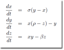
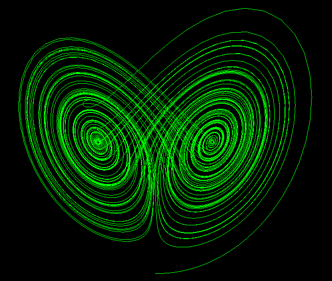
Perhaps the iconic figure that springs to mind when thinking about Chaos Theory, this attractor is born of a set of non-linear differential equations derived from simplified versions of equations used to model the weather.
System of Equations
| Function Syntax | lorenz |
| Current Version | 1.1 |
| Compatible with AutoCAD for Mac? | Yes |
| Compatible with AutoCAD LT? | Yes |
| Donate |
;; Lorenz Attractor  -  Lee Mac

(defun c:lorenz ( / a b c h n x x0 y y0 z z0 )
    (setq
        n  10000 ;; Iterations
        h  0.01  ;; Increment
        a  10.0  ;; sigma
        b  28.0  ;; rho
        c  (/ 8.0 3.0) ;; beta

        x0 0.1   ;;
        y0 0.0   ;; Initial values
        z0 0.0   ;;
    )
    (entmake '((0 . "POLYLINE") (70 . 8)))
    (repeat n
        (setq
            x (+ x0 (* h a (- y0 x0)))
            y (+ y0 (* h (- (* x0 (- b z0)) y0)))
            z (+ z0 (* h (- (* x0 y0) (* c z0))))
            x0 x
            y0 y
            z0 z
        )
        (entmake (list '(0 . "VERTEX") '(70 . 32) (list 10 x y z)))
    )
    (entmake '((0 . "SEQEND")))
    (princ)
)
Result
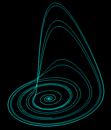
The Rössler Attractor
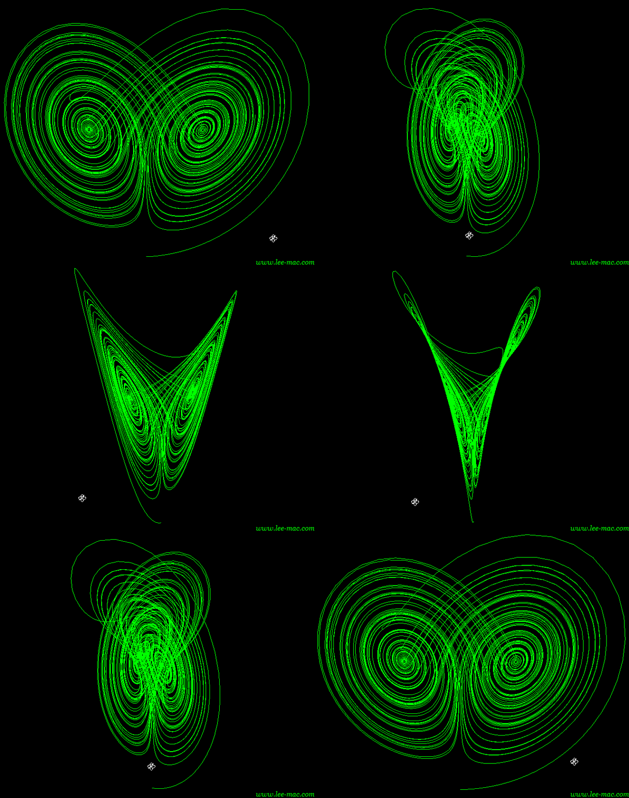
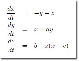
Designed by Otto Rössler in 1976, this set of three non-linear ordinary differential equations was later found to be useful in modelling equilibrium in chemical reactions.
System of Equations
| Function Syntax | rossler |
| Current Version | 1.1 |
| Compatible with AutoCAD for Mac? | Yes |
| Compatible with AutoCAD LT? | Yes |
| Donate |
;; Rössler Attractor  -  Lee Mac

(defun c:rossler ( / a b c h n x x0 y y0 z z0 )
    (setq
        n  10000 ;; Iterations
        h  0.01  ;; Increment
        a  0.2
        b  0.2
        c  5.7

        x0 0.1   ;;
        y0 0.0   ;; Initial values
        z0 0.0   ;;
    )
    (entmake '((0 . "POLYLINE") (70 . 8)))
    (repeat n
        (setq
            x (+ x0 (* h (- (- y0) z0)))
            y (+ y0 (* h (+ x0 (* a y0))))
            z (+ z0 (* h (+ b (* z0 (- x0 c)))))
            x0 x
            y0 y
            z0 z
        )
        (entmake (list '(0 . "VERTEX") '(70 . 32) (list 10 x y z)))
    )
    (entmake '((0 . "SEQEND")))
    (princ)
)
Result
The Duffing Oscillator
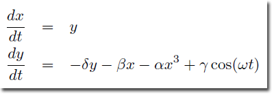
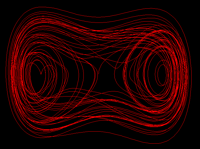
This system, named after George Duffing, is used to model a damped oscillator such as a weighted non-uniform spring. The system is described by the following non-linear second-order differential equation, aptly known as the Duffing Equation:

For those not versed in mathematical shorthand notation, the above equation may be alternatively written as:

Here, δ is the damping force, α is the force exerted by the spring (the 'restoring force'), β introduces the non-uniform nature of the spring (for β = 0 we have a damped & driven simple harmonic oscillator - far less exciting!), γ is the size of the driving force (i.e. the weight on the spring), and ω is the frequency of the driving force.
To solve the Duffing Equation using a numerical method, I have reduced the above second-order differential equation into a system of two first-order differential equations:
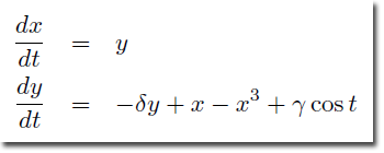
Finally, to obtain the chaotic attractor, I have set α = 1, β = -1, & ω = 1, resulting in the following system in which we may vary δ & γ:
| Function Syntax | duffing |
| Current Version | 1.1 |
| Compatible with AutoCAD for Mac? | Yes |
| Compatible with AutoCAD LT? | Yes |
| Donate |
;; Duffing Attractor  -  Lee Mac

(defun c:duffing ( / a b h l n tt x x0 y y0 )
    (setq
        n  10000 ;; Iteratons
        h  0.04  ;; Increment
        a  0.2   ;; delta
        b  0.3   ;; gamma

        x0 0.0   ;;
        y0 0.0   ;; Initial values
        tt 0.0   ;;
    )
    (entmake
        (append
            (list
               '(000 . "LWPOLYLINE")
               '(100 . "AcDbEntity")
               '(100 . "AcDbPolyline")
                (cons 90 n)
               '(70 . 0)
            )
            (repeat n
                (setq
                    x  (+ x0 (* h y0))
                    y  (+ y0 (* h (+ (- x0 (* x0 x0 x0) (* a y0)) (* b (cos tt)))))
                    tt (+ tt h)
                    x0 x
                    y0 y
                    l  (cons (list 10 x y) l)
                )
            )
        )
    )
    (princ)
)
Result
Instructions for Running
Please refer to How to Run an AutoLISP Program.
