
Logistic Map
I've always been fascinated by this ostensibly simple map, which produces astoundingly complex dynamics resulting in chaos if a single parameter is varied.
I have hence constructed a couple of programs to demonstrate this interesting behaviour.
A Brief Overview of the Logistic Map
The Logistic map was originally devised as a population model, to measure the growth of a population, noting that the rate of reproduction of a species is proportional to the existing population and restricted by the available resources and competition for such resoures.
The study involves iterating the following difference equation:
x[n] = rx[n](1-x[n])
For varying values of 0 <= r <= 4 and 0 <= x[0] <= 1
The function maximum occurs at r/4, hence for 0 <= r <= 4, values of x in the interval [0,1] remain in [0,1]. The function diverges for values of r outside of [0,4].
For 0 <= r <= 1 we have a single fixed point at x=0
For 1 < r <= 3 we have two fixed points at x=0 (unstable, repellor) and x=(r-1)/r (attractor)
As r approaches 3, convergence to the fixed point x=(r-1)/r becomes increasingly slow, and a periodic point of period 2 appears when 3 < r < 1+sqrt(6) (approx. 3.45).
From here we have a period-doubling cascade with the period doubling at a rate of approximately 4.669 (the Feigenbaum Constant).
For r > 3.57 chaos emerges, with 'islands of stability' for various values of r at which periods of order 5,6,7 emerge.
For r=4 the interval [0,1] is mapped to a set resembling a Cantor Set, with Hausdorff Dimension of about 0.538.
A Visual Study of the Logistic Map
| Function Syntax | Logistic |
| Current Version | 1.0 |
| Download | Logistic.lsp / Logistic.dcl |
| View HTML Version | Logistic.html |
| Compatible with AutoCAD for Mac? | Yes |
| Compatible with AutoCAD LT? | Yes |
| Donate |
To view the general dynamics of the Logistic Map, I have created a program where the parameter r and the initial state x can be varied, and the long-term behaviour of the model is displayed.
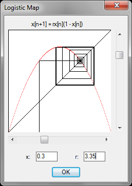
Notice that, as the parameter r is increased, the behaviour becomes extremely complex, resulting in a chaotic state at r=4.
Bifurcation Diagram
| Function Syntax | LogisticB |
| Current Version | 1.0 |
| Download | LogisticB.lsp / LogisticB.dcl |
| View HTML Version | LogisticB.html |
| Compatible with AutoCAD for Mac? | Yes |
| Compatible with AutoCAD LT? | Yes |
| Donate |
The long term behaviour of the solution for each value of the parameter r can also be mapped, forming what is known as a 'Bifurcation Diagram'.
Upon viewing such a diagram it is clear that the solution branches at those values of the parameter for which the period doubles in the above program, resulting in chaos for around 3.57 onwards.
Another interesting observation are the 'islands of stability': the strips of uniform behaviour at approximately 3.63, 3.74 and 3.82.
Further Examples of Chaotic Maps
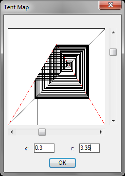
It may be demonstrated that chaotic behaviour displayed by the Logistic Map arises in any map with a single peak in the interval [0,1].
To illustrate this fact with my program, the iterated function may be altered to display other maps:
The Tent Map
(setq f (lambda ( x ) (if (< x 0.5) (* 0.5 r x) (* 0.5 r (- 1 x)))))
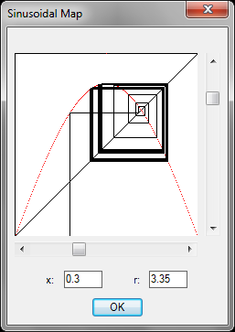
A Sinusoidal Map
(setq f (lambda ( x ) (* 0.25 r (sin (* pi x)))))
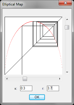
An Elliptical Map
(setq f (lambda ( x ) (* 0.5 r (sqrt (* (- x) (1- x))))))
Instructions for Running
- Download both the LISP and DCL files from the links above.
- Ensure the DCL file is located in an AutoCAD Support Path.
- Load the LISP file. (refer to How to Run an AutoLISP Program).
- Type the noted Function Syntax at the AutoCAD command-line to run the program.